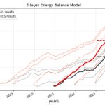





ALT Surface temp anomalies (a) observed in 2023 and (b) simulated by the trop Pacific pacemaker simulation with a global climate model.


ALT Diurnal cycle of land surface temperature (LST) difference between the city of Warsaw and its rural surroundings, for (a) the summer months (JJA) during clear-sky conditions (5-year mean). The IFS 4.4 km simulations are given with red lines (Cycle 2 dashed, Cycle 3 solid), and observations from LSA SAF are given in black. The bottom panels show JJA-mean clear-sky LST anomaly maps at 13:00 local time, with respect to the surrounding rural LST average, for (b) observations from LSA SAF, (c) IFS 4.4 km Cycle 3 with the urban scheme, and (d) IFS 4.4 km in Cycle 2 without the urban scheme and using older land use–land cover maps.


ALT Imprint of simulated Arctic sea ice leads on 2 m temperature in the Laptev Sea and East Siberian Sea. (a) Sea ice concentration field and (b) 2 m temperature field. The panels depict 13 February 2020, at 08:00, in the IFS-FESOM Cycle 3 simulation with TCo2559 (4.4 km), coupled to the NG5 ocean (∼ 4–5 km resolution in this area). The black and white contour lines represent the border between land and ocean areas.

ALT Eddy variability expressed as the standard deviation of daily SSH data. The left column shows data from the Cycle 3 simulation of IFS-FESOM model, while the right column shows AVISO multi-satellite altimeter data. In AVISO, the global mean SSH is removed from each grid point. AVISO data consist of the time period 2017–2021, while 2020–2024 is used for IFS-FESOM.

ALT Snapshot for 31 January 2020 at 21:00 UTC of infrared brightness temperature (left) and hourly precipitation rate (right) over the Indian Ocean, from (a) observations (Meteosat 8 SEVIRI channel 9 and GPM IMERG) and on forecast day 12 of (b) IFS-NEMO 4.4 km and (c) 9 km (third row) simulations. The simulations use the nextGEMS Cycle 3 setup except that they are run with a satellite image simulator and, for technical reasons, are coupled to NEMO V3.4 (ORCA025) here.

ALT Global-mean TOA imbalance as a function of global-mean surface air temperature (GSAT). Grey lines show the climatological range of individual CERES years (2001–2020) over ERA5 GSAT data (Hersbach et al., 2020). Thin lines are tracing monthly mean values, with a small square marking the final month for each simulation. Big squares depict annual means (dashed for Cycle 2, solid for Cycle 3), and for multi-year simulations, thick solid lines are tracing annual means for each year, with the big square marking the last simulated annual mean.